A common problem in digital image processing is detecting straight lines. The brute force solution is to test every point for lines. This approach is computationally intensive.
The Hough transform reduces the amount of computation to detect lines by transforming the x and y plane to a theta and p plane. For straight lines, we can use this equation:
p = x * cos * theta + y * sin * theta
For every x and y coordinate, the value of p is calculated for a specific interval of radians from 0 to $\pi$. The example in the paper uses 20 degree intervals. The results of these calculations are then stored in an accumulator table, which counts the number of occurrences for p and $\theta$ pairs. Pairs with the most occurrences are a good indicator of a straight line. The threshold can be adjusted manually to count straight lines.
The downside of this approach is that it does not seem to find all straight lines and is somewhat dependent on the edge detection algorithm used. In addition, the performance - although much improved from the brute force solution - is still slow. This is true especially on larger images combined with small radian intervals.
Hough transform implementation
Fig. 1 Linear Hough transform on airplane with OpenCV
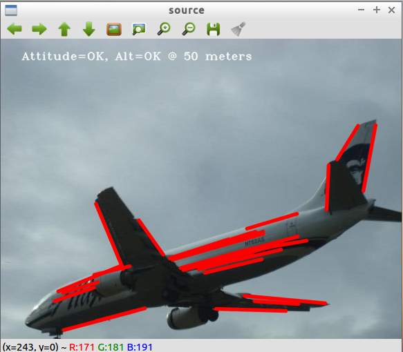
The Alaska Airlines airplane image was a good choice since there are obvious straight lines. The algorithm does a good job find most of the lines.
Fig. 2 Canny edge detection on airplane before linear Hough transform with OpenCV
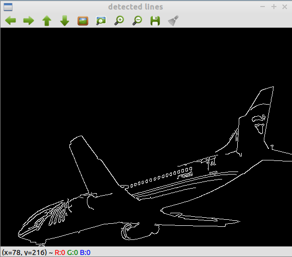
The Canny detection image gives a good the accuracy of the Hough transform. Particularly interesting is the lower half of the plane’s body. There are no lines there at all. At first, this seemed like an error, but that part of the plane is curved. As will be shown later, my naive implementation of the hough transform messes up on this part. This seems to be one of the improvements with the probabilistic hough transform. OpenCV’s implementation has a parameter for minimum line length.
There are some errors in the transform though, mainly at the head of the plane and the windows. The probabilistic hough transform function of Open CV (HoughTransformP) contains parameters to control the maximum line gap, so it’s possible the gap value was set too high. In the example code, it is set to 10 pixels.
Fig. 3 Naive Hough transform on airplane
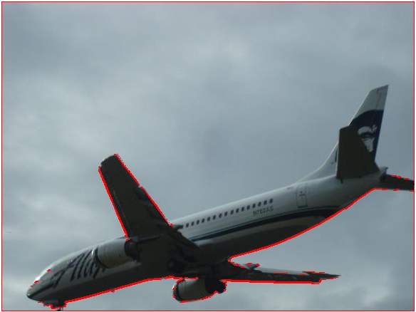
Fig. 4 Sobel transform applied on airplane before Hough transform
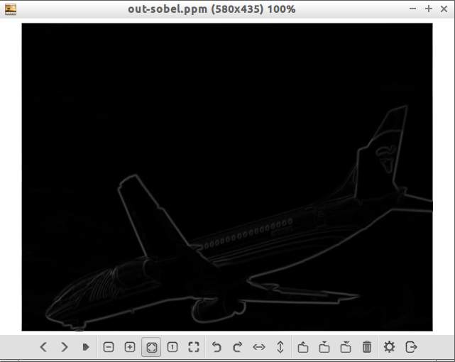
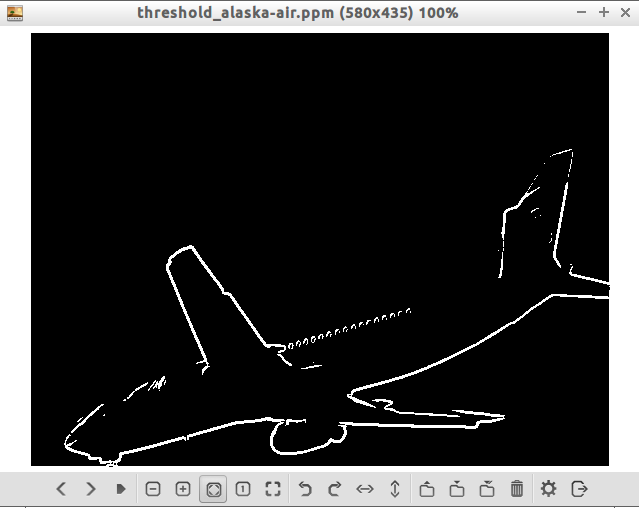
Fig. 5 Threshold applied after Sobel on airplane before Hough transform
In order to understand the Hough Transform more thoroughly, I attempted to implement the algorithm based on the paper in exercise 1 and the explanations in “Digital Image Processing” by Gonzalez and Woods.
My implementation was very basic and bare bones. From Fig. 3, it can be seen that lines in the tail of the plane are not worked and that the lower body of the plane is considered an entire line. This may be because my implementation does not take gaps into account. It’s also not clear why the tail of the plane is not marked since those edges were detected by the Sobel transform. Sobel was used in place of Canny since my Canny implementation needs more work.
For the Sobel transform, one improvement I learned from looking at the GIMP implementation is dividing the final gradient (not sure if this is the right term) by 5.66. This seems to lessen the intensity of the colors and makes lighter lines black and removes a lot of noise. Relevant snippet of code:
data_out[i][j] = (UINT8)(sqrt(grad_x * grad_x + grad_y * grad_y) / 5.66);