Chapter 4 of the “Practical Deep Learning for Coders” course leaves the full digit classifier as an exercise for the reader. This post walks through my solution.
Data wrangling
I will skip most of the details for setting up the data since most of that is similar to what was described in the previous post for the two digit classifier. See appendix A for the general set up code.
Appendix A also sets up a testing dataset to check against overfitting.
The only major change is with the format for the labels. In the two digit example, we created a tensor with a shape of torch.Size([11693, 1], but in this exercise, the shape will be torch.Size([60000]. This is because we’re using a different loss function, specifically the Pytorch implementation of cross entropy loss. That’s just how the function expects the tensor to be formatted.
Basically:
[1, 2, 3]
Instead of:
[
    [1], [2], [3]
]
Cross entropy loss
We’re using cross entropy loss since it allows us to handle more than two possible labels, which I think is called multiclass classification (different than multilabel classification which allows multiple labels to be selected for a given example).
I also looked into other strategies, such as “one versus rest” and “one versus one,” but they seemed less efficient than the cross entropy loss approach. These two strategies try to turn the multiclass classification into multiple different binary classification problems. This can lead to a large number of variations.
I don’t fully understand the math for how cross entropy loss works yet, but intuitively it seems like it will generate probabilities for each of the possibilities, then we pick the label with the highest probability. The sum of the probabilities of each possibility will add up to one.
Chapter 5 of the “Practical Deep Learning for Coders” course has an in-depth explanation of how cross entropy loss works. There are also some good articles online that I found helpful.
Generalized model code
One drawback of using Jupyter notebooks is that the usage of cells makes it harder to write reusable code. This code snippet is a cleaned up version of the code described in the previous post.
def train_model(train_dataset, valid_dataset, model, optimizer, epochs):
    for i in range(epochs):
        train_epoch(model, train_dataset, optimizer)
        # Was using this for checking the performance of the model after each epoch
        print(validate_epoch(model, valid_dataset), end="  ")


def train_epoch(model, train_dataset, optimizer):
    for xb, yb in train_dataset:
        calc_grad(xb, yb, model)
        optimizer.step()
        optimizer.zero_grad()


def calc_grad(xb, yb, model):
    preds = model(xb)
    loss = loss_func(preds, yb)
    loss.backward()


def validate_epoch(model, valid_dataset):
    accs = [batch_accuracy(model(xb), yb) for xb, yb in valid_dataset]
    return round(torch.stack(accs).mean().item(), 4)


def batch_accuracy(xb, yb):
    # Normalize predictions (I think my use of the sigmoid function is wrong here)
    preds = xb.sigmoid()
    # Pick the index that is has the highest value
    _, indices = torch.max(preds, 1)
    correct = indices == yb
    return correct.float().mean()
Simple linear model
The first model I tried was a simple linear model that takes 784 inputs (28x28) and returns 10 outputs.
lr = 0.01
epochs = 400
num_outputs = len(digits_paths)
linear_model = nn.Linear(28 * 28, num_outputs)
opt = SGD(linear_model.parameters(), lr)
loss_func = nn.CrossEntropyLoss()

train_model(train_dataset, valid_dataset, linear_model, opt, epochs)
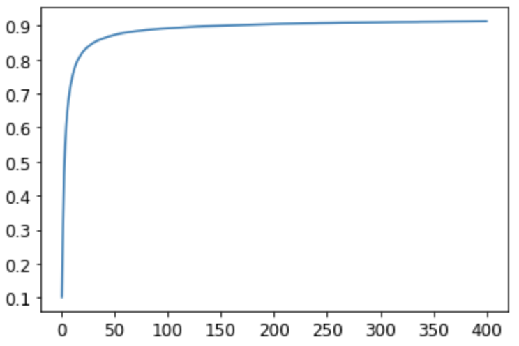
The performance over 400 epochs was 0.9126 which is decent, but seems like we can do better.
Here’s a graph of the accuracy over each epoch. The performance improvements starts steep, but very quickly flattens out.

Two layer model
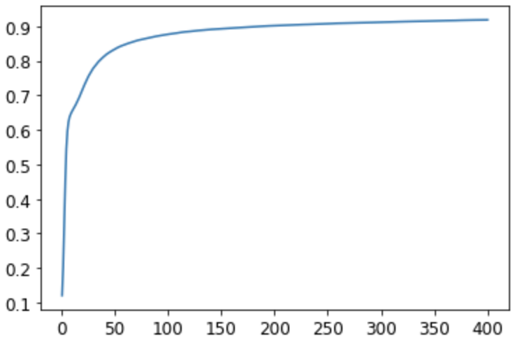
Next I tried a two layer model over the same 400 epochs. This model also tailed off around 91% accuracy. It didn’t seem to matter how many inputs I used for the second layer. The 30 I picked here is arbitrary. My main observation here is that this model performed worse than the simple linear model when I used fewer epochs. The improvement in accuracy seems to improve slower. But I’m not sure why. I did use a smaller learning rate. And also the model is slightly more complex.
lr_simple = 0.001
epochs = 400
simple_net = nn.Sequential(
    nn.Linear(28*28, 30),
    nn.ReLU(),
    nn.Linear(30, num_outputs),
)
opt_simple = SGD(simple_net.parameters(), lr_simple)

train_model(train_dataset, valid_dataset, simple_net, opt_simple, epochs)

Three layer model
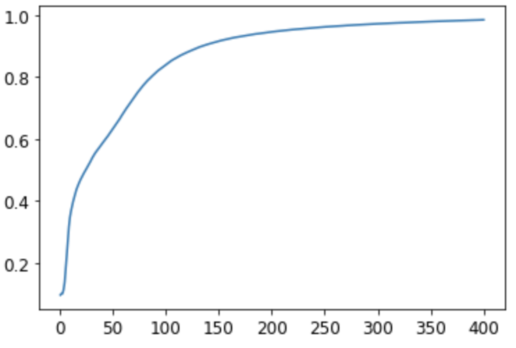
The last model I tried was a three layer model. Much like the two layer model I experimented with different inputs and outputs as well epochs. In my initial tests, I ran the model over 40 epochs and 160 epochs. It was concerning that the performance was always noticeably worse than the simple linear model. But once I increased the epochs to 400, the three layer model’s performance reached 0.9845. The accuracy improved slower, but more steadily than the two layer model.
lr_simple_3 = 0.01
epochs = 400
simple_net_3 = nn.Sequential(
    nn.Linear(28*28, 300),
    nn.ReLU(),
    nn.Linear(300, 50),
    nn.ReLU(),
    nn.Linear(50, num_outputs),
)
opt_simple_3 = SGD(simple_net_3.parameters(), lr_simple_3)

train_model(train_dataset, valid_dataset, simple_net_3, opt_simple_3, epochs)

Performance against the testing dataset
To help ensure that I hadn’t overfitted the models, I ran the models against the testing data provided by the MNIST data set. The results looked reasonable.
print(validate_epoch(linear_model, testing_dataset))
print(validate_epoch(simple_net, testing_dataset))
print(validate_epoch(simple_net_4, testing_dataset))

0.9165
0.9201
0.9713
The Fast.AI model
Finally I also tested out the performance using the Fast.AI library code. It was able to reach an accuracy 0.984 in one epoch, which took 12 minutes to run.
path2 = untar_data(URLs.MNIST)
Path.BASE_PATH = path2

dls = ImageDataLoaders.from_folder(path2, train='training', valid_pct=0.2)
learn = cnn_learner(dls, resnet18, pretrained=False, loss_func=F.cross_entropy, metrics=accuracy)
learn.fit_one_cycle(1, 0.1)

Appendix A: Setting up data
# Load MNIST data
path = untar_data(URLs.MNIST)
Path.BASE_PATH = path

# Load all digit paths
digits_paths = [
	(path/"training"/str(digit)).ls().sorted()
	for digit in range(10)
]

# Convert images to tensors
digit_tensors = [
    [tensor(Image.open(f)) for f in paths]
    for paths in digits_paths
]

# Convert each digit list into one tensor
stacked_digits = [
    torch.stack(digits).float()/255
    for digits in digit_tensors
]

# Combine all digits
digits_x = torch.cat(stacked_digits).view(-1, 28 * 28)
digits_y = tensor(
    list(chain.from_iterable([[i] * len(paths) for i, paths in enumerate(digits_paths)]))
)
dataset = list(zip(digits_x, digits_y))

# Create validation set
mini_batch_size = 256
valid_split = 0.2
split_index = int(len(digits_x) * valid_split)
shuffled_indices = torch.randperm(len(digits_x))
train_indices, valid_indices = shuffled_indices[split_index:], shuffled_indices[:split_index]

train_sampler = SubsetRandomSampler(train_indices)
valid_sampler = SubsetRandomSampler(valid_indices)

train_dataset = DataLoader(dataset, batch_size=mini_batch_size, sampler=train_sampler)
valid_dataset = DataLoader(dataset, batch_size=mini_batch_size, sampler=valid_sampler)

# Set up testing dataset
testing_paths = [(path/"testing"/str(digit)).ls().sorted() for digit in range(10)]
testing_tensors = [
    [tensor(Image.open(f)) for f in paths]
    for paths in testing_paths
]
stacked_testing = [
    torch.stack(digits).float()/255
    for digits in testing_tensors
]
testing_x = torch.cat(stacked_testing).view(-1, 28 * 28)
testing_y = tensor(
    list(chain.from_iterable([[i] * len(paths) for i, paths in enumerate(testing_paths)]))
)
testing_dataset_temp = list(zip(testing_x, testing_y))
testing_dataset = DataLoader(testing_dataset_temp, batch_size=256)